# We use the PCMBase package to do basic manipulation with trees and models.
# See https://venelin.github.io/PCMBase for an introduction into this package.
library(PCMBase)
library(PCMBayes)
library(ggtree)

# The PCMBase package comes with a collection of simulated objects, which we
# can use as example.

tree <- PCMBaseTestObjects$tree.ab
model <- PCMExtractDimensions(PCMBaseTestObjects$model_MixedGaussian_ab, dims = 1:2)
X <- PCMBaseTestObjects$traits.ab.123[1:2, ]

# Plot the tree and the data
plTree <- PCMTreePlot(tree) +
  geom_tiplab(size = 3) + geom_nodelab(nudge_x = .02, nudge_y = 2, size = 2) +
  theme_tree2()
plData <- PCMPlotTraitData2D(
  X[, seq_len(PCMTreeNumTips(tree))],
  labeledTips = seq_len(PCMTreeNumTips(tree)),
  sizeLabels = 3,
  sizePoints = 1,
  nudgeLabels = c(0.4, 0.4),
  tree, numTimeFacets = 3, scaleSizeWithTime = FALSE)

cowplot::plot_grid(plTree, plData, nrow = 2)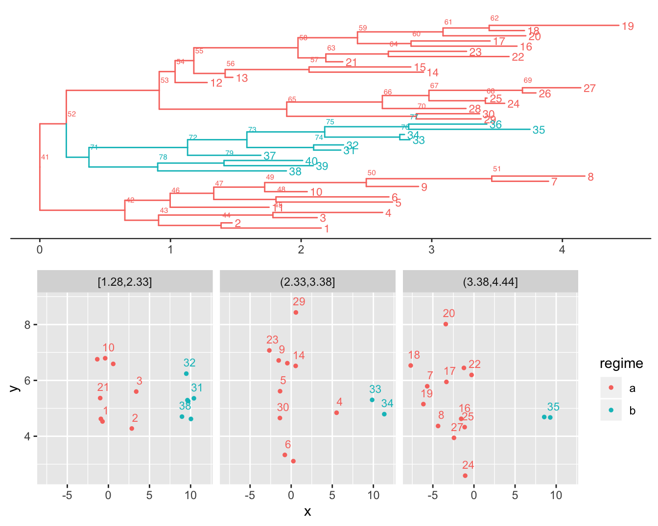
mgpmTemplate <- MixedGaussian(
  k = 2,
  modelTypes = MGPMDefaultModelTypes(),
  mapping = structure(1:6, names = LETTERS[1:6]),
  Sigmae_x = Args_MixedGaussian_MGPMDefaultModelTypes()$Sigmae_x)

# Set a Gaussian prior for the initial state X0
PCMAddPrior(mgpmTemplate, member = "X0", enclos = "?",
         prior = ParameterPrior(d = "dnorm", r = "rnorm",
                                p = list(mean = c(4, 2), sd = c(2, 2))))

# Set a uniform prior for the elements of H and Sigma_x such that all elements
# are in the interval [-4, 4]. Later we overwrite this prior for the diagonal
# elements of H and Sigma_x.
PCMAddPrior(
  mgpmTemplate, member = "H|Sigma_x", enclos = "?",
  prior = ParameterPrior(d = "dunif", r = "runif", p = list(min = -4, max = 4)))

# Set exponential priors for the (non-negative) diagonal elements of the OU
# selection strength matrix H and the BM/OU matrix parameter Sigma_x. Note that,
# we are using class _Schur for the H matrix. That's why the diagonal elements
# of the untransformed matrix H are equal to the eigenvalues of the actual
# selection strength matrix obtained after transformation. For the matrix
# Sigma_x the diagonal elements denote the standard deviation of the unit-time
# drift of the traits.
# Note that this prior setting overwrites the uniform prior for the diagonal
# elements we have set previously -- the order of the AddPrior commands is
# important.
PCMAddPrior(mgpmTemplate, member = "H|Sigma_x", enclos = "diag(?[,,1])",
         prior = ParameterPrior(d = "dexp", r = "rexp", p = list(rate = 10)))

# Set a Gaussian prior for the OU-parameter Theta:
PCMAddPrior(mgpmTemplate, member = "Theta", enclos = "?",
         prior = ParameterPrior(d = "dnorm", r = "rnorm",
                                p = list(mean = c(8, 2), sd = c(4, 2))))

# Now we create the context object
ctx <- MCMCContext(X, tree, mgpmTemplate)

state <- MCMCState(s = c(
  3,              # K: number of shifts
  52, 46, 73,     # n_2, ..., n_{K+1}: shift nodes
  0.1, 0.4, 0.3,  # l_2, ..., l_{K+1}: offsets of the shift points relative
                  # to the beginnings of shift branches in tip-ward direction.
  52, 46, 41,     # r_2,...,r_{K+1}: regime indices corresponding to the shifts.
                  # The regime of the part starting at the root node (41) is
                  # set to 41 (not included in the list). The regime for the
                  # part 73 is again 41, meaning that this regime is lumped with
                  # the root regime. So the number of regimes is R=3.
  5, 2, 2         # model type mapping for the three regimes.
  ), ctx)

priorObj <- PCMPrior(state$model)
PriorDensity(priorObj, state$v)
## [1] -2.038575 0.000000 0.000000 0.000000 0.000000 0.000000 0.000000
## [8] 0.000000 0.000000 0.000000 0.000000 0.000000 0.000000 0.000000
## [15] 0.000000 0.000000