Getting started with the PCMFit R-package
Venelin Mitov
2021-06-05
Source:vignettes/ResultsBootstrap/MGPM_A_F_BC2_RR_BSID_1/vignettes/pcmfit.Rmd
pcmfit.RmdNote: The writing of this vignette is currently in progress. If needed, please, contact the author for assistance. Thanks for your understanding.
Using the PCMFit R-package comprises several steps:
- Preparing the data, to which we wish to fit phylogenetic comparative model (PCM);
- Deciding on the type of PCM we wish to infer;
- Defining the PCM;
- Calling a PCMFit model inference function on the data and model type we have defined;
- Evaluating the inferred model.
Before we start, let’s load the packages needed for this tutorial:
library(PCMBase)
library(PCMFit)
library(data.table)
library(ggplot2)
library(ggtree)
library(cowplot)

# make results reproducible
set.seed(4, kind = "Mersenne-Twister", normal.kind = "Inversion")
In the next sections, we go through each of the above steps:
Step 1. An example dataset
For this tutorial, we will use a simulated non-ultrametric tree of \(N=80\) tips and simulated \(k=2\)-variate trait values. Both of these are stored in the data-table dtSimulated included with the PCMFit package.
The data
We use the PCMBase::PCMTreePlot() and PCMBase::PCMPlotTraitData2D() functions to generate plots of the tree and the data (note that PCMBase::PCMTreePlot() requires the ggtree R-package which is currently not on CRAN - see the ggtree home page for instructions how to install this package):
plTree <- PCMTreePlot(tree, layout="fan") +
  geom_tiplab2(size = 2) +
  geom_nodelab(size = 2, color = "black") +
  geom_treescale(width = max(PCMTreeNodeTimes(tree)), x = 0, linesize = .25, fontsize = 2, offset = 79)

plX <- PCMPlotTraitData2D(
  X[, seq_len(PCMTreeNumTips(tree))],
  tree,
  scaleSizeWithTime = FALSE,
  numTimeFacets = 4) +
  geom_text(
    aes(x = x, y = y, label = id, color = regime),
    size=2,
    position = position_jitter(.4, .4)) +
  theme_bw() +
  theme(legend.position = "bottom")

cowplot::plot_grid(plTree, plX, labels = LETTERS[1:2], nrow=2, rel_heights = c(2,1))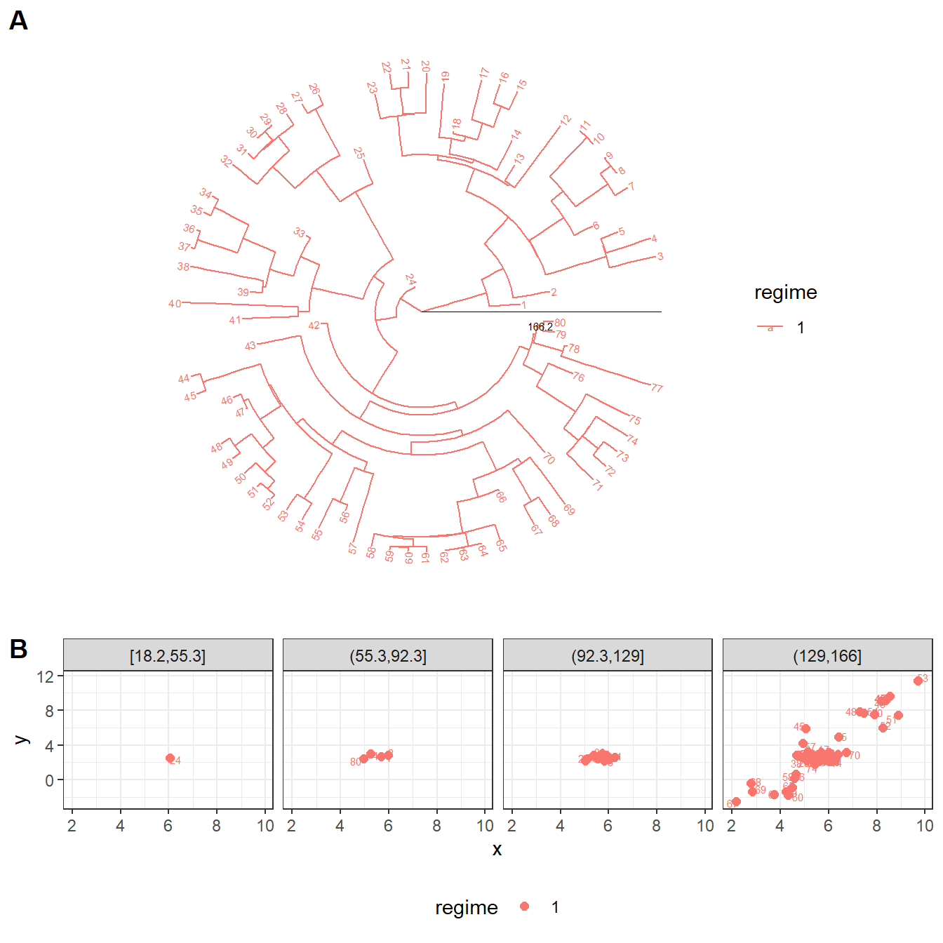
Example phylogenetic comparative data. A: a tree of 80 tips. B: bivariate trait values at the tips of the tree.
Step 2. Gaussian model types
In this tutorial, we use the six model types \(BM_{A}\), \(BM_{B}\), \(OU_{C}\), \(OU_{D}\), \(OU_{E}\), \(OU_{F}\) from the \(\mathcal{G}_{LInv}\)-family as defined in (Mitov, Bartoszek, and Stadler 2019). These model types are also described in the PCMBase Getting started guide:
# scroll to the right in the following listing to see the aliases for the six
# default model types:
PCMDefaultModelTypes()
#>                                                                                                                                                                                A
#>                                                                                                      "BM__Global_X0__Diagonal_WithNonNegativeDiagonal_Sigma_x__Omitted_Sigmae_x"
#>                                                                                                                                                                                B
#>                                                                                   "BM__Global_X0__UpperTriangularWithDiagonal_WithNonNegativeDiagonal_Sigma_x__Omitted_Sigmae_x"
#>                                                                                                                                                                                C
#>                                       "OU__Global_X0__Schur_Diagonal_WithNonNegativeDiagonal_Transformable_H__Theta__Diagonal_WithNonNegativeDiagonal_Sigma_x__Omitted_Sigmae_x"
#>                                                                                                                                                                                D
#>                    "OU__Global_X0__Schur_Diagonal_WithNonNegativeDiagonal_Transformable_H__Theta__UpperTriangularWithDiagonal_WithNonNegativeDiagonal_Sigma_x__Omitted_Sigmae_x"
#>                                                                                                                                                                                E
#> "OU__Global_X0__Schur_UpperTriangularWithDiagonal_WithNonNegativeDiagonal_Transformable_H__Theta__UpperTriangularWithDiagonal_WithNonNegativeDiagonal_Sigma_x__Omitted_Sigmae_x"
#>                                                                                                                                                                                F
#>                             "OU__Global_X0__Schur_WithNonNegativeDiagonal_Transformable_H__Theta__UpperTriangularWithDiagonal_WithNonNegativeDiagonal_Sigma_x__Omitted_Sigmae_x"
Our purpose for this tutorial will be to select an optimal model for the data. We will compare “global” models in which one model of one of the above model types is fit to the entire tree and data, versus a mixed Gaussian phylogenetic model where different models of the above model types are assigned to different parts of the tree.
Step 3. Creating model objects
Global models
A global \(BM_{B}\) model
modelBM <- PCM(
  PCMDefaultModelTypes()["B"], modelTypes = PCMDefaultModelTypes(), k = 2)

modelBM
#> Brownian motion model
#> S3 class: BM__Global_X0__UpperTriangularWithDiagonal_WithNonNegativeDiagonal_Sigma_x__Omitted_Sigmae_x, BM, GaussianPCM, PCM; k=2; p=5; regimes: 1. Parameters/sub-models:
#> X0 (VectorParameter, _Global, numeric; trait values at the root):
#> [1] 0 0
#> Sigma_x (MatrixParameter, _UpperTriangularWithDiagonal, _WithNonNegativeDiagonal; factor of the unit-time variance rate):
#> , , 1
#>
#>      [,1] [,2]
#> [1,]    0    0
#> [2,]    0    0
#>
#> Sigmae_x (MatrixParameter, _Omitted; factor of the non-heritable variance or the variance of the measurement error):
#>
#>
A global \(OU_{F}\) model
modelOU <- PCM(
  PCMDefaultModelTypes()["F"], modelTypes = PCMDefaultModelTypes(), k = 2)

modelOU
#> Ornstein-Uhlenbeck model
#> S3 class: OU__Global_X0__Schur_WithNonNegativeDiagonal_Transformable_H__Theta__UpperTriangularWithDiagonal_WithNonNegativeDiagonal_Sigma_x__Omitted_Sigmae_x, OU, GaussianPCM, PCM, _Transformable; k=2; p=11; regimes: 1. Parameters/sub-models:
#> X0 (VectorParameter, _Global, numeric; trait values at the root):
#> [1] 0 0
#> H (MatrixParameter, _Schur, _WithNonNegativeDiagonal, _Transformable; adaptation rate matrix):
#> , , 1
#>
#>      [,1] [,2]
#> [1,]    0    0
#> [2,]    0    0
#>
#> Theta (VectorParameter, matrix; long-term optimum):
#>      1
#> [1,] 0
#> [2,] 0
#> Sigma_x (MatrixParameter, _UpperTriangularWithDiagonal, _WithNonNegativeDiagonal; factor of the unit-time variance rate):
#> , , 1
#>
#>      [,1] [,2]
#> [1,]    0    0
#> [2,]    0    0
#>
#> Sigmae_x (MatrixParameter, _Omitted; factor of the non-heritable variance or the variance of the measurement error):
#>
#>
MGPM models
A MGPM with the true shift-point configuration and model type mapping
modelTrueTypeMapping <- MixedGaussian(
  k = 2,
  modelTypes = MGPMDefaultModelTypes(),
  mapping = c(4, 3, 2),
  X0 = structure(
    0, class = c("VectorParameter",
                 "_Global"), description = "trait values at the root"),
  Sigmae_x = structure(
    0, class = c("MatrixParameter", "_Omitted",
                 "_Global"),
    description =
      "Upper triangular Choleski factor of the non-phylogenetic variance-covariance"))

treeWithTrueShifts <- PCMTree(PCMFitDemoObjects$dtSimulated$tree[[1]])
PCMTreeSetPartRegimes(
  treeWithTrueShifts,
  part.regime = c(`81` = 1, `105` = 2, `125` = 3),
  setPartition = TRUE)
A MGPM with the true shift-point configuration, model type mapping and parameter values
modelTrue <- PCMFitDemoObjects$dtSimulated$model[[1]]
modelTrue
#> Mixed Gaussian model
#> S3 class: MixedGaussian_432, MixedGaussian, GaussianPCM, PCM, _Transformable; k=2; p=18; regimes: 1, 2, 3. Parameters/sub-models:
#> X0 (VectorParameter, _Global, numeric; trait values at the root):
#> [1]  1 -1
#> 1 (OU__Omitted_X0__Schur_Diagonal_WithNonNegativeDiagonal_Transformable_H__Theta__UpperTriangularWithDiagonal_WithNonNegativeDiagonal_Sigma_x__Omitted_Sigmae_x, OU, GaussianPCM, PCM, _Transformable):
#> Ornstein-Uhlenbeck model
#> S3 class: OU__Omitted_X0__Schur_Diagonal_WithNonNegativeDiagonal_Transformable_H__Theta__UpperTriangularWithDiagonal_WithNonNegativeDiagonal_Sigma_x__Omitted_Sigmae_x, OU, GaussianPCM, PCM, _Transformable; k=2; p=7; regimes: 1. Parameters/sub-models:
#> X0 (VectorParameter, _Omitted; trait values at the root):
#>
#> H (MatrixParameter, _Schur, _Diagonal, _WithNonNegativeDiagonal, _Transformable; adaptation rate matrix):
#> , , 1
#>
#>      [,1] [,2]
#> [1,] 1.39 0.00
#> [2,] 0.00 0.59
#>
#> Theta (VectorParameter, matrix; long-term optimum):
#>         1
#> [1,] 5.94
#> [2,] 2.58
#> Sigma_x (MatrixParameter, _UpperTriangularWithDiagonal, _WithNonNegativeDiagonal; Choleski factor of the unit-time variance rate):
#> , , 1
#>
#>      [,1] [,2]
#> [1,] 0.29 0.02
#> [2,] 0.00 0.36
#>
#> Sigmae_x (MatrixParameter, _Omitted; Choleski factor of the non-heritable variance or the variance of the measurement error):
#>
#>
#> 2 (OU__Omitted_X0__Schur_Diagonal_WithNonNegativeDiagonal_Transformable_H__Theta__Diagonal_WithNonNegativeDiagonal_Sigma_x__Omitted_Sigmae_x, OU, GaussianPCM, PCM, _Transformable):
#> Ornstein-Uhlenbeck model
#> S3 class: OU__Omitted_X0__Schur_Diagonal_WithNonNegativeDiagonal_Transformable_H__Theta__Diagonal_WithNonNegativeDiagonal_Sigma_x__Omitted_Sigmae_x, OU, GaussianPCM, PCM, _Transformable; k=2; p=6; regimes: 1. Parameters/sub-models:
#> X0 (VectorParameter, _Omitted; trait values at the root):
#>
#> H (MatrixParameter, _Schur, _Diagonal, _WithNonNegativeDiagonal, _Transformable; adaptation rate matrix):
#> , , 1
#>
#>      [,1] [,2]
#> [1,] 0.37 0.00
#> [2,] 0.00 1.06
#>
#> Theta (VectorParameter, matrix; long-term optimum):
#>         1
#> [1,] 5.41
#> [2,] 2.63
#> Sigma_x (MatrixParameter, _Diagonal, _WithNonNegativeDiagonal; Choleski factor of the unit-time variance rate):
#> , , 1
#>
#>      [,1] [,2]
#> [1,] 0.36  0.0
#> [2,] 0.00  0.4
#>
#> Sigmae_x (MatrixParameter, _Omitted; Choleski factor of the non-heritable variance or the variance of the measurement error):
#>
#>
#> 3 (BM__Omitted_X0__UpperTriangularWithDiagonal_WithNonNegativeDiagonal_Sigma_x__Omitted_Sigmae_x, BM, GaussianPCM, PCM):
#> Brownian motion model
#> S3 class: BM__Omitted_X0__UpperTriangularWithDiagonal_WithNonNegativeDiagonal_Sigma_x__Omitted_Sigmae_x, BM, GaussianPCM, PCM; k=2; p=3; regimes: 1. Parameters/sub-models:
#> X0 (VectorParameter, _Omitted; trait values at the root):
#>
#> Sigma_x (MatrixParameter, _UpperTriangularWithDiagonal, _WithNonNegativeDiagonal; Choleski factor of the unit-time variance rate):
#> , , 1
#>
#>      [,1] [,2]
#> [1,] 0.17 0.14
#> [2,] 0.00 0.50
#>
#> Sigmae_x (MatrixParameter, _Omitted; Choleski factor of the non-heritable variance or the variance of the measurement error):
#>
#>
#> Sigmae_x (MatrixParameter, _Omitted; upper triangular Choleski factor of the non-phylogenetic variance-covariance):
#>
#>

# We specify the tree and trait values for the true model in order to easily
# calculate parameter count likelihood and AIC for it:
attr(modelTrue, "tree") <- treeWithTrueShifts
attr(modelTrue, "X") <- X
attr(modelTrue, "SE") <- X * 0.0
A view of the data according to the true shift-point configuration
plTree <- PCMTreePlot(treeWithTrueShifts, layout="fan") %<+%
  data.table(
    node = c(12, 77, 45),
    part.model = c(" 1.D ", " 2.C ", " 3.B "),
    offset = 5) +
  geom_tiplab2(size = 2) +
  geom_tiplab2(aes(label = part.model), offset = 16) +
  geom_nodelab(size = 2, color = "black") +
  geom_treescale(
    width = max(PCMTreeNodeTimes(treeWithTrueShifts)), x = 0,
    linesize = .25, fontsize = 2, offset = 79)

plX <- PCMPlotTraitData2D(
  X[, seq_len(PCMTreeNumTips(treeWithTrueShifts))],
  treeWithTrueShifts,
  scaleSizeWithTime = FALSE,
  numTimeFacets = 4) +
  geom_text(
    aes(x = x, y = y, label = id, color = regime),
    size=2,
    position = position_jitter(.4, .4)) +
  theme_bw() +
  theme(legend.position = "bottom")

cowplot::plot_grid(plTree, plX, labels = LETTERS[1:2], nrow = 2, rel_heights = c(2,1))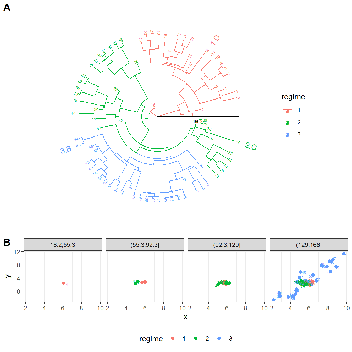
Example phylogenetic comparative data. A: a tree of 80 tips partitioned in three evolutionary regimes. Each evolutionary regime is denoted by #.T, where # is the regime identifier and T is the evolutionary model type associated with this regime (a model type among A, …, F). B: bivariate trait values at the tips of the tree.
Step 4. Model inference
Specifying parameter limits
An optional but important preliminary step is to explicitly specify the limits for the model parameters. This is needed, because the default settings might not be appropriate for the data in question. Here is an example how the model parameter limits can be set. Note that we specify these limits for the base “BM” and “OU” model types, but they are inherited by their subtypes A, …, F, as specified in the comments.
## File: DefineParameterLimits.R
# lower limits for models A and B
PCMParamLowerLimit.BM <- function(o, k, R, ...) {
  o <- NextMethod()
  k <- attr(o, "k", exact = TRUE)
  R <- length(attr(o, "regimes", exact = TRUE))

  if(is.Global(o$Sigma_x)) {
    if(!is.Diagonal(o$Sigma_x)) {
      o$Sigma_x[1, 2] <- -.0
    }
  } else {
    if(!is.Diagonal(o$Sigma_x)) {
      for(r in seq_len(R)) {
        o$Sigma_x[1, 2, r] <- -.0
      }
    }
  }
  o
}

# upper limits for models A and B
PCMParamUpperLimit.BM <- function(o, k, R, ...) {
  o <- NextMethod()
  k <- attr(o, "k", exact = TRUE)
  R <- length(attr(o, "regimes", exact = TRUE))

  if(is.Global(o$Sigma_x)) {
    o$Sigma_x[1, 1] <- o$Sigma_x[2, 2] <- 1.0
    if(!is.Diagonal(o$Sigma_x)) {
      o$Sigma_x[1, 2] <- 1.0
    }
  } else {
    for(r in seq_len(R)) {
      o$Sigma_x[1, 1, r] <- o$Sigma_x[2, 2, r] <- 1.0
      if(!is.Diagonal(o$Sigma_x)) {
        o$Sigma_x[1, 2, r] <- 1.0
      }
    }
  }
  o
}

# lower limits for models C, ..., F.
PCMParamLowerLimit.OU <- function(o, k, R, ...) {
  o <- NextMethod()
  k <- attr(o, "k", exact = TRUE)
  R <- length(attr(o, "regimes", exact = TRUE))

  if(is.Global(o$Theta)) {
    o$Theta[1] <- 0.0
    o$Theta[2] <- -1.2
  } else {
    for(r in seq_len(R)) {
      o$Theta[1, r] <- 0.0
      o$Theta[2, r] <- -1.2
    }
  }
  if(is.Global(o$Sigma_x)) {
    if(!is.Diagonal(o$Sigma_x)) {
      o$Sigma_x[1, 2] <- -.0
    }
  } else {
    if(!is.Diagonal(o$Sigma_x)) {
      for(r in seq_len(R)) {
        o$Sigma_x[1, 2, r] <- -.0
      }
    }
  }
  o
}

# upper limits for models C, ..., F.
PCMParamUpperLimit.OU <- function(o, k, R, ...) {
  o <- NextMethod()
  k <- attr(o, "k", exact = TRUE)
  R <- length(attr(o, "regimes", exact = TRUE))

  if(is.Global(o$Theta)) {
    o$Theta[1] <- 7.8
    o$Theta[2] <- 4.2
  } else {
    for(r in seq_len(R)) {
      o$Theta[1, r] <- 7.8
      o$Theta[2, r] <- 4.2
    }
  }
  if(is.Global(o$Sigma_x)) {
    o$Sigma_x[1, 1] <- o$Sigma_x[2, 2] <- 1.0
    if(!is.Diagonal(o$Sigma_x)) {
      o$Sigma_x[1, 2] <- 1.0
    }
  } else {
    for(r in seq_len(R)) {
      o$Sigma_x[1, 1, r] <- o$Sigma_x[2, 2, r] <- 1.0
      if(!is.Diagonal(o$Sigma_x)) {
        o$Sigma_x[1, 2, r] <- 1.0
      }
    }
  }
  o
}
Fitting an MGPM model with known shift-point configuration and model type mapping but unknown model parameters
# This can take about 5 minutes to finish
fitMGPMTrueTypeMapping <- PCMFit(
  model = modelTrueTypeMapping,
  tree = treeWithTrueShifts,
  X = X,
metaI = PCMBaseCpp::PCMInfoCpp)Step 5. Evaluating the model fits
listModels <- list(
  RetrieveBestModel(fitBM),
  RetrieveBestModel(fitOU),
  RetrieveBestModel(fitMGPMTrueTypeMapping),
  RetrieveBestModel(fitMGPMTrueTypeMappingCheat),
  modelTrue)

dtSummary <- data.table(
  model = c(
    "Global BM",
    "Global OU",
    "True MGPM, unknown parameters",
    "True MGPM, known true parameters",
    "True MGPM, true parameters"),
  p = sapply(listModels, PCMParamCount),
  logLik = sapply(listModels, logLik),
  AIC = sapply(listModels, AIC))
knitr::kable(dtSummary)| model | p | logLik | AIC |
|---|---|---|---|
| Global BM | 5 | -221.68133 | 455.3627 |
| Global OU | 11 | -204.60164 | 433.2033 |
| True MGPM, unknown parameters | 18 | -93.65584 | 233.3117 |
| True MGPM, known true parameters | 18 | -93.50648 | 233.0130 |
| True MGPM, true parameters | 18 | -102.63502 | 251.2700 |
References
Mitov, Venelin, Krzysztof Bartoszek, and Tanja Stadler. 2019. “Automatic Generation of Evolutionary Hypotheses Using Mixed Gaussian Phylogenetic Models.” Proceedings of the National Academy of Sciences of the United States of America. https://www.pnas.org/lookup/doi/10.1073/pnas.1813823116.