Here, we introduce the R-package POUMM - an implementation of the Phylogenetic Ornstein-Uhlenbeck Mixed Model (POUMM) for univariate continuous traits (Mitov and Stadler 2018, 2019). In the sections below, we demonstrate how the package works. To that end, we run a simulation of a trait according to the POUMM model. Then, we execute a maximum likelihood (ML) and a Bayesian (MCMC) POUMM fit to the simulated data. We show how to use plots and some diagnostics to assess the quality of the fit, i.e. the mixing and the convergence of the MCMC, as well as the consistency of the POUMM fit with the true POUMM parameters from the simulation. Once you are familiar with these topics, we recommend reading the vignette Interpreting the POUMM.

But before we start, we need to install and load a few R-packages from CRAN:

install.packages("data.table")
install.packages("ggplot2")
install.packages("lmtest")
install.packages("ape")

library(ggplot2)
library(data.table)
library(lmtest)
library(ape)

Installing the POUMM R-package

You can install the most recent version of the package from github:

devtools::install_github(repo="venelin/POUMM")

The above command will install the HEAD version from the master git-branch. This is the package branch, which evolves the fastest and gets the quickest bug-fixes.

A more stable version of the package can be installed from CRAN:

install.packages("POUMM")

The above commands will install all 3rd party dependencies with one exception: the package for high precision floating point arithmetics (Rmpfr). While the POUMM can be run without Rmpfr installed, installing this package is recommended to prevent numerical instability in some extreme cases, i.e. very small positive values for the POUMM parameters alpha, sigma, and sigmae. Currently, Rmpfr is listed as “Suggests” in POUMM’s DESCRIPTION, since it’s installation has been problematic on some systems (i.e. Linux). If you have not done this before, you may need to enable Rcpp in your R environment. You can read how to do this in the Rcpp-FAQ vignette available from this page.

Bear in mind that, for CRAN compliance, some of the functionality of the package might not be enabled on some systems, in particular, parallel likelihood calculation on Mac OS X El Capitan using clang compiler prior to version 6 (see the section Parallel execution below).

Simulating trait evolution under the POUMM

Parameters of the simulation

First, we specify the parameters of the POUMM simulation:

N <- 500
g0 <- 0           
alpha <- .5        
theta <- 2        
sigma <- 0.2     
sigmae <- 0.2

We briefly explain the above parameters. The first four of them define an OU-process with initial state $g_0$, a selection strength parameter, $\alpha$, a long-term mean, $\theta$, and a stochastic time-unit standard deviation, $\sigma$. To get an intuition about the OU-parameters, one can consider random OU-trajectories using the function rTrajectoryOU(). On the figure below, notice that doubling $\alpha$ speeds up the convergence of the trajectory towards $\theta$ (magenta line) while doubling $\sigma$ results in bigger stochastic oscilations (blue line):

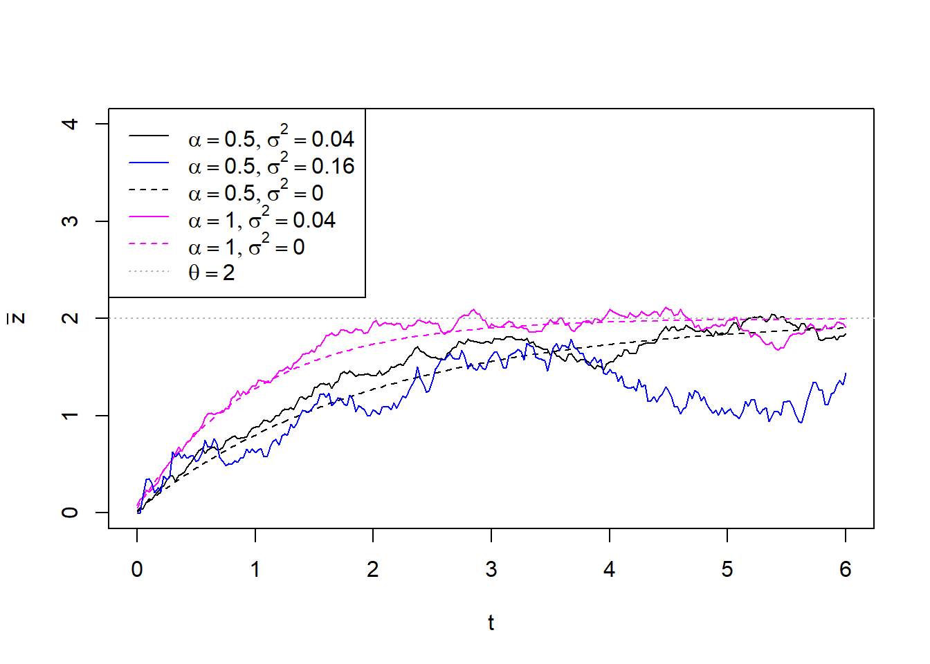
$Dashed black and magenta lines denote the deterministic trend towards the long-term mean $\theta$, fixing the stochastic parameter $\sigma=0$.$

Dashed black and magenta lines denote the deterministic trend towards the long-term mean $\theta$, fixing the stochastic parameter $\sigma=0$.

The POUMM models the evolution of a continuous trait, $z$, along a phylogenetic tree, assuming that $z$ is the sum of a genetic (heritable) component, $g$, and an independent non-heritable (environmental) component, $e\sim N(0,\sigma_e^2)$. At every branching in the tree, the daughter lineages inherit the $g$-value of their parent, adding their own environmental component $e$. The POUMM assumes the genetic component, $g$, evolves along each lineage according to an OU-process with initial state the $g$ value inherited from the parent-lineage and global parameters $\alpha$, $\theta$ and $\sigma$.

Simulating the phylogeny

Once the POUMM parameters are specified, we use the ape R-package to generate a random tree with 500 tips:

# Number of tips
tree <- rtree(N)

plot(tree, show.tip.label = FALSE)

Simulating trait evolution on the phylogeny

Starting from the root value $g_0$, we simulate the genotypic values, $g$, and the environmental contributions, $e$, at all internal nodes down to the tips of the phylogeny:

# genotypic (heritable) values
g <- rVNodesGivenTreePOUMM(tree, g0, alpha, theta, sigma)

# environmental contributions
e <- rnorm(length(g), 0, sigmae)

# phenotypic values
z <- g + e

Visualizing the data

In most real situations, only the phenotypic value, at the tips, i.e. will be observable. One useful way to visualize the observed trait-values is to cluster the tips in the tree according to their root-tip distance, and to use box-whisker or violin plots to visualize the trait distribution in each group. This allows to visually assess the trend towards uni-modality and normality of the values - an important prerequisite for the POUMM.

# This is easily done using the nodeTimes utility function in combination with
# the cut-function from the base package.
data <- data.table(z = z[1:N], t = nodeTimes(tree, tipsOnly = TRUE))
data <- data[, group := cut(t, breaks = 5, include.lowest = TRUE)]

ggplot(data = data, aes(x = t, y = z, group = group)) + 
  geom_violin(aes(col = group)) + geom_point(aes(col = group), size=.5)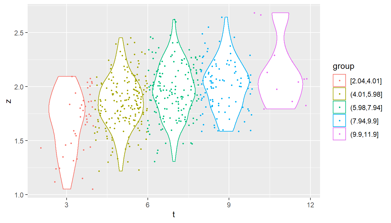

Distributions of the trait-values grouped according to their root-tip distances.

Fitting the POUMM

Once all simulated data is available, it is time proceed with a first POUMM fit. This is done easily by calling the function POUMM():

fitPOUMM <- POUMM(z[1:N], tree)

The above code runs for about 5 minutes on a MacBook Pro Retina (late 2013) with a 2.3 GHz Intel Core i7 processor. Using default settings, it performs a maximum likelihood (ML) and a Bayesian (MCMC) fit to the data. First the ML-fit is done. Then, three MCMC chains are run as follows: the first MCMC chain samples from the default prior distribution, i.e. assuming a constant POUMM likelihood; the second and the third chains perform adaptive Metropolis sampling from the posterior parameter distribution conditioned on the default prior and the data. By default each chain is run for $10^5$ iterations. This and other default POUMM settings are described in the help-page for the function specifyPOUMM().

The strategy of executing three MCMC chains instead of one allows to assess:

the quality of the MCMC fit: a mismatch between the sampling distributions of the second and third chains suggests that at least one of the chains has not converged to a region of high posterior density (HPD).
the presence of signal for the POUMM parameters in the data: a close match between prior and posterior distributions suggests lack of signal in the data.

We plot traces and posterior sample densities from the MCMC fit:

# get a list of plots 
plotList <- plot(fitPOUMM, showUnivarDensityOnDiag = TRUE, doPlot = FALSE)
plotList$traceplot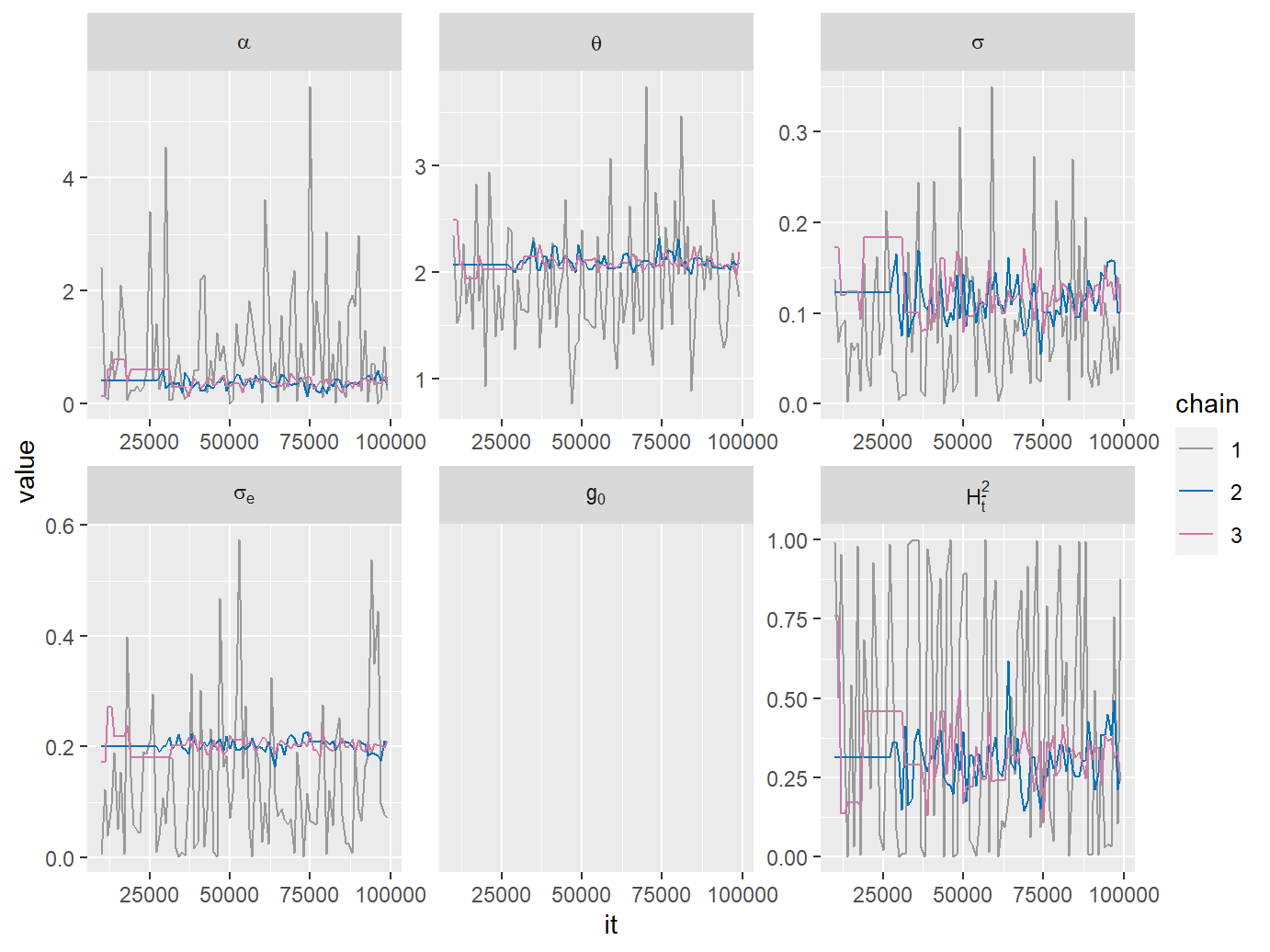

MCMC traces from a POUMM MCMC-fit.

plotList$densplot

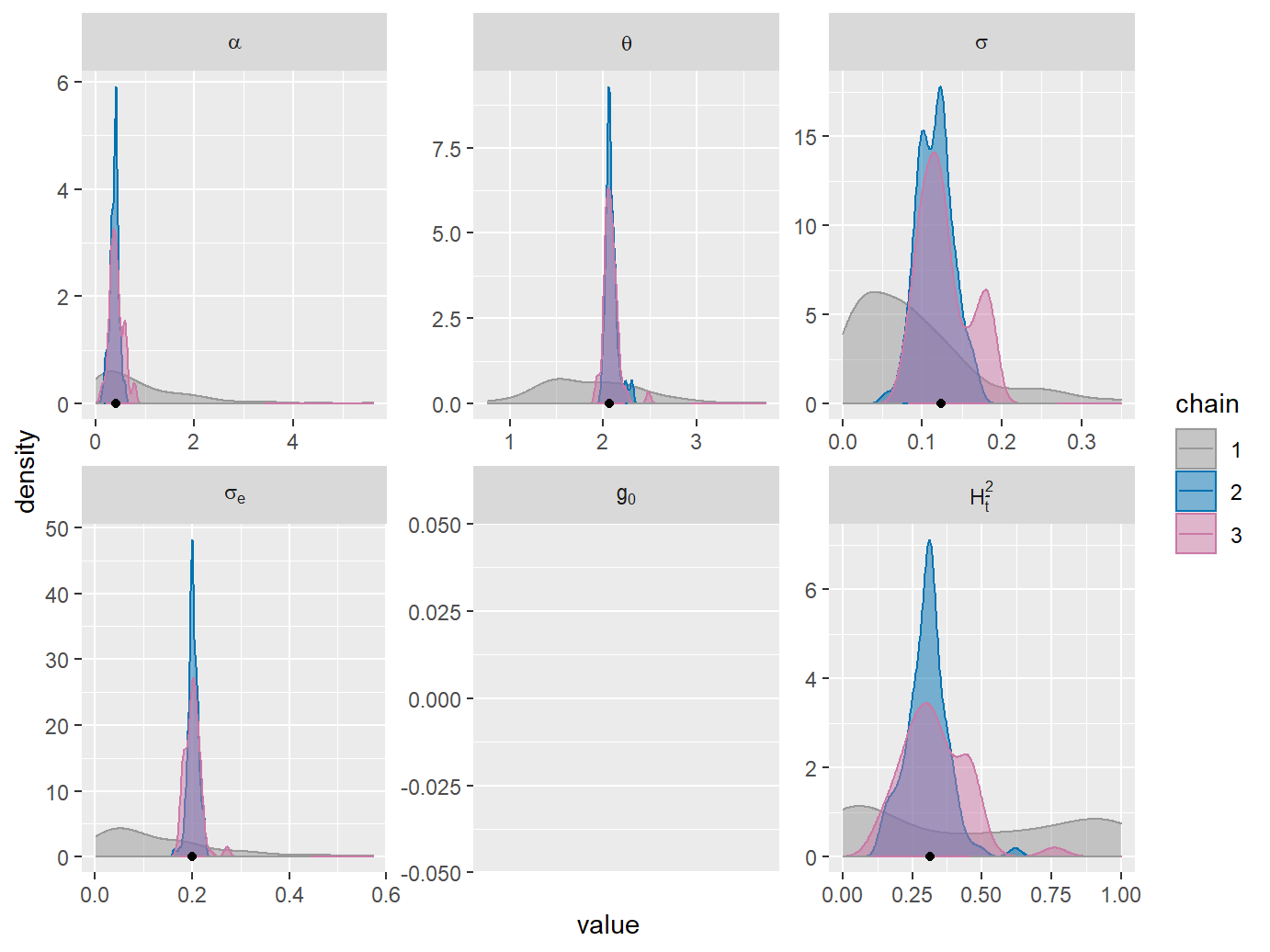
MCMC univariate density plots. Black dots on the x-axis indicate the ML-fit.

A mismatch of the posterior sample density plots from chains 2 and 3, in particular for the phylogenetic heritability, $H_{\bar{t}}^2$, indicates that the chains have not converged. This can be confirmed quantitatively by the Gelman-Rubin statistic (column called G.R.) in the summary of the fit:

summary(fitPOUMM)

##             stat   N       MLE PostMean               HPD    ESS  G.R.
##  1:        alpha 500   0.41430  0.40221     0.1898,0.6705  77.34 1.126
##  2:        theta 500   2.06446  2.08657       1.958,2.248 128.33 1.030
##  3:        sigma 500   0.12321  0.12200   0.07823,0.17237  78.51 1.119
##  4:       sigmae 500   0.19983  0.20199     0.1779,0.2252  99.72 1.083
##  5:          H2e 500   0.43886  0.42389     0.2871,0.5550  99.58 1.100
##  6:       H2tInf 500   0.31451  0.31965     0.1278,0.4446 131.32 1.102
##  7:       H2tMax 500   0.31450  0.31935     0.1278,0.4445 131.24 1.100
##  8:      H2tMean 500   0.31343  0.31641     0.1267,0.4429 130.67 1.096
##  9:           g0 500        NA       NA             NA,NA   0.00    NA
## 10: sigmaG2tMean 500   0.01823  0.01961 0.007174,0.029110 148.95 1.205
## 11:  sigmaG2tMax 500   0.01832  0.02005 0.007235,0.029455 151.11 1.225
## 12:  sigmaG2tInf 500   0.01832  0.02013 0.007236,0.029464 154.32 1.232
## 13:      logpost 500        NA 14.28151      1.609,17.014  36.65 1.315
## 14:       loglik 500  16.32733       NA             NA,NA   0.00    NA
## 15:          AIC 500 -22.65466       NA             NA,NA   0.00    NA
## 16:         AICc 500 -22.53320       NA             NA,NA   0.00    NA

The G.R. diagnostic is used to check whether two random samples originate from the same distribution. Values that are substantially different from 1.00 (in this case greater than 1.01) indicate significant difference between the two samples and possible need to increase the number of MCMC iterations. Therefore, we rerun the fit specifying that each chain should be run for $4 \times 10^5$ iterations:

fitPOUMM2 <- POUMM(z[1:N], tree, spec=list(nSamplesMCMC = 4e5))

Now, both the density plots and the G.R. values indicate nearly perfect convergence of the second and third chains. The agreement between the ML-estimates (black dots on the density plots) and the posterior density modes (approximate location of the peak in the density curves) shows that the prior does not inflict a bias on the MCMC sample. The mismatch between chain 1 and chains 2 and 3 suggests that the information about the POUMM parameters contained in the data disagrees with or significantly improves our prior knowledge about these parameters. This is the desired outcome of a Bayesian fit, in particular, in the case of a weak (non-informed) prior, such as the default one.

plotList <- plot(fitPOUMM2, doPlot = FALSE)
plotList$densplot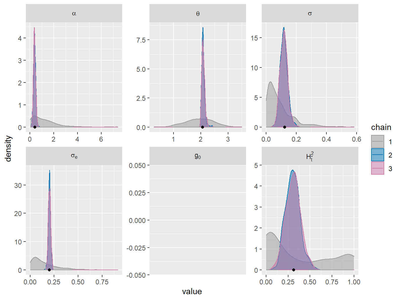

summary(fitPOUMM2)

##             stat   N       MLE PostMean               HPD    ESS   G.R.
##  1:        alpha 500   0.41430  0.38942     0.2104,0.5747  720.0 1.0015
##  2:        theta 500   2.06446  2.08602       1.987,2.195  720.0 1.0009
##  3:        sigma 500   0.12321  0.11770   0.07336,0.16939  720.0 0.9986
##  4:       sigmae 500   0.19983  0.20191     0.1802,0.2286  799.1 0.9994
##  5:          H2e 500   0.43886  0.42494     0.2658,0.5435  799.5 0.9999
##  6:       H2tInf 500   0.31451  0.30849     0.1470,0.4694 1274.0 1.0015
##  7:       H2tMax 500   0.31450  0.30831     0.1468,0.4694 1273.0 1.0015
##  8:      H2tMean 500   0.31343  0.30572     0.1437,0.4679 1263.7 1.0013
##  9:           g0 500        NA       NA             NA,NA    0.0     NA
## 10: sigmaG2tMean 500   0.01823  0.01815 0.009029,0.030213 1266.7 1.0053
## 11:  sigmaG2tMax 500   0.01832  0.01838 0.008773,0.030115 1264.1 1.0058
## 12:  sigmaG2tInf 500   0.01832  0.01840 0.008774,0.030178 1264.3 1.0057
## 13:      logpost 500        NA 15.02485       12.17,17.07  720.0 1.0013
## 14:       loglik 500  16.32733       NA             NA,NA    0.0     NA
## 15:          AIC 500 -22.65466       NA             NA,NA    0.0     NA
## 16:         AICc 500 -22.53320       NA             NA,NA    0.0     NA

Consistency of the fit with the “true” simulation parameters

The 95% high posterior density (HPD) intervals contain the true values for all five POUMM parameters ($\alpha$, $\theta$, $\sigma$, $\sigma_e$ and $g_0$). This is also true for the derived statistics. To check this, we calculate the true derived statistics from the true parameter values and check that these are well within the corresponding HPD intervals:

tMean <- mean(nodeTimes(tree, tipsOnly = TRUE))
tMax <- max(nodeTimes(tree, tipsOnly = TRUE))

c(# phylogenetic heritability at mean root-tip distance: 
  H2tMean = H2(alpha, sigma, sigmae, t = tMean),
  # phylogenetic heritability at long term equilibirium:
  H2tInf = H2(alpha, sigma, sigmae, t = Inf),
  # empirical (time-independent) phylogenetic heritability, 
  H2e = H2e(z[1:N], sigmae),
  # genotypic variance at mean root-tip distance: 
  sigmaG2tMean = varOU(t = tMean, alpha, sigma),
  # genotypic variance at max root-tip distance: 
  sigmaG2tMean = varOU(t = tMax, alpha, sigma),
  # genotypic variance at long-term equilibrium:
  sigmaG2tInf = varOU(t = Inf, alpha, sigma)
  )

##      H2tMean       H2tInf          H2e sigmaG2tMean sigmaG2tMean  sigmaG2tInf 
##      0.49958      0.50000      0.43792      0.03993      0.04000      0.04000

Finally, we compare the ratio of empirical genotypic to total phenotypic variance with the HPD-interval for the phylogenetic heritability.

c(H2empirical = var(g[1:N])/var(z[1:N]))

## H2empirical 
##      0.6541

summary(fitPOUMM2)["H2e"==stat, unlist(HPD)]

##  lower  upper 
## 0.2658 0.5435

Parallel execution

On computers with multiple core processors, it is possible to speed-up the POUMM-fit by parallelization. The POUMM package supports parallelization on two levels:

parallelizing the POUMM likelihood calculation. The POUMM package parallelizes the likelihood calculation through the SPLITT library for parallel lineage traversal (Mitov and Stadler 2019). This is a fine grain parallelization, which can benefit from modern single instruction multiple data (SIMD) processors as well as multiple physical cores. Parallelization on multiple cores becomes beneficial on trees exceeding several hundreds tips. For this parallelization to work, the POUMM package must be compiled from source-code using an OpenMP 4.0-enabled C++ compiler. Open MP 4.0 is supported by several modern C++ compilers including Gnu-g++, Intel-icpc and clang version 6.0 or above (see also the SPLITT Get started guide for details).

To control the maximum number of threads (defaults to all physical or virtual cores on the system) by specifying the environment variable OMP_NUM_THREADS, before starting R e.g.:

export OMP_NUM_THREADS=4

parallelizing the MCMC-chains - this can be done by creating a cluster using the R-package parallel. With the default settings of the MCMC-fit (executing two MCMC chains sampling from the posterior distribution and one MCMC chain sampling from the prior), this parallelization can result in about two times speed-up of the POUMM fit on a computer with at least two available physical cores.

# set up a parallel cluster on the local computer for parallel MCMC:
cluster <- parallel::makeCluster(parallel::detectCores(logical = FALSE))
doParallel::registerDoParallel(cluster)

fitPOUMM <- POUMM(z[1:N], tree, spec=list(parallelMCMC = TRUE))

# Don't forget to destroy the parallel cluster to avoid leaving zombie worker-processes.
parallel::stopCluster(cluster)

It is possible to use this parallelization in combination with parallelization of the likelihood calculation. This, however, has not been tested and, presumably, would be slower than a parallelization on the likelihood level only. It may be appropriate to parallelize the MCMC chains on small trees, since for small trees, the parallel likelihood calculation is not likely to be much faster than a serial mode calculation. In this case the SPLITT library would switch automatically to serial mode, so there will be no parallel CPU at the likelihood level.

Packages used

Apart from base R functionality, the POUMM package uses a number of 3rd party R-packages:

For likelihood calculation: Rcpp v1.0.3 (Eddelbuettel et al. 2017), Rmpfr v0.8.1 (Maechler 2016);
For mcmcSampling: adaptMCMC v1.3 (Scheidegger 2012);
For MCMC convergence diagnostics, calculation of MCMC effective sizes and HPD-intervals: coda v0.19.3 (Plummer et al. 2016);
For other purposes (parameter transformations and summary statistics): parallel v3.6.3 (Team, n.d.), foreach v1.4.8 (Revolution Analytics and Weston, n.d.), data.table v1.13.2 (Dowle and Srinivasan 2016), Matrix v1.2.18 (Bates and Maechler 2017));
For tree processing: ape v5.3 (Paradis et al. 2016);
For reporting: data.table v1.13.2 (Dowle and Srinivasan 2016), ggplot2 v3.3.0 (Wickham and Chang 2016), lmtest v0.9.38 (Hothorn et al. 2015);
For testing: testthat v2.3.2 (Wickham 2016), mvtnorm v1.1.0 (Genz et al. 2016).

References

Bates, Douglas, and Martin Maechler. 2017. Matrix: Sparse and Dense Matrix Classes and Methods. https://CRAN.R-project.org/package=Matrix.

Dowle, Matt, and Arun Srinivasan. 2016. Data.table: Extension of ‘Data.frame‘. https://CRAN.R-project.org/package=data.table.

Eddelbuettel, Dirk, Romain Francois, JJ Allaire, Kevin Ushey, Qiang Kou, Nathan Russell, Douglas Bates, and John Chambers. 2017. Rcpp: Seamless R and C++ Integration. https://CRAN.R-project.org/package=Rcpp.

Genz, Alan, Frank Bretz, Tetsuhisa Miwa, Xuefei Mi, and Torsten Hothorn. 2016. Mvtnorm: Multivariate Normal and T Distributions. https://CRAN.R-project.org/package=mvtnorm.

Hothorn, Torsten, Achim Zeileis, Richard W. Farebrother, and Clint Cummins. 2015. Lmtest: Testing Linear Regression Models. https://CRAN.R-project.org/package=lmtest.

Maechler, Martin. 2016. Rmpfr: R Mpfr - Multiple Precision Floating-Point Reliable. https://CRAN.R-project.org/package=Rmpfr.

Mitov, Venelin, and Tanja Stadler. 2018. “A Practical Guide to Estimating the Heritability of Pathogen Traits.” Molecular Biology and Evolution 35 (3): 756–72. https://doi.org/10.1093/molbev/msx328.

———. 2019. “Parallel Likelihood Calculation for Phylogenetic Comparative Models: The Splitt C++ Library.” Methods in Ecology and Evolution. https://doi.org/10.1111/2041-210X.13136.

Paradis, Emmanuel, Simon Blomberg, Ben Bolker, Julien Claude, Hoa Sien Cuong, Richard Desper, Gilles Didier, et al. 2016. Ape: Analyses of Phylogenetics and Evolution. https://CRAN.R-project.org/package=ape.

Plummer, Martyn, Nicky Best, Kate Cowles, Karen Vines, Deepayan Sarkar, Douglas Bates, Russell Almond, and Arni Magnusson. 2016. Coda: Output Analysis and Diagnostics for Mcmc. https://CRAN.R-project.org/package=coda.

Revolution Analytics, and Steve Weston. n.d. Foreach: Provides Foreach Looping Construct for R.

Scheidegger, Andreas. 2012. AdaptMCMC: Implementation of a Generic Adaptive Monte Carlo Markov Chain Sampler. https://CRAN.R-project.org/package=adaptMCMC.

Team, R Core. n.d. Support for Parallel Computation in R.

Wickham, Hadley. 2016. Testthat: Unit Testing for R. https://CRAN.R-project.org/package=testthat.

Wickham, Hadley, and Winston Chang. 2016. Ggplot2: Create Elegant Data Visualisations Using the Grammar of Graphics. https://CRAN.R-project.org/package=ggplot2.

A User Guide to the POUMM R-package

Venelin Mitov