Simulating epidemics with the toyepidemic R-package
Venelin Mitov
Designing the epidemic
Define the pathogen genotypes
We set the numbers of different alleles for each quantitative trait locus (QTL) in the pathogen genotype. These are specified in the form of a integer vector with elements bigger or equal to 2. The length of this vector corresponds to the number of QTLs.
# numbers of alleles for each quantitative trait locus
numsAllelesAtSites <- c(3, 2)

# Define a matrix of the possible genotype encodings (as allele contents).
genotypes <- generateGenotypes(numsAllelesAtSites)
print(genotypes)
## [,1] [,2]
## [1,] 1 1
## [2,] 1 2
## [3,] 2 1
## [4,] 2 2
## [5,] 3 1
## [6,] 3 2# Define the probability of the first infecting strain (the first pathogen strain starting the epidemic)
pg.init <- rep(0, nrow(genotypes))
pg.init[1] <- 1 # we specify that 1 is the first strain with probability 1.Define the number and the frequencies of host-types
# number of host-types
n <- 6

# probability of each host type in a susceptible compartment
pe <- runif(n)
pe <- pe/sum(pe) # ensure that they sum-up to 1
Define the GE-values
The GE-values represent the general genotype x host-type effects. A genotype x host-type effect is the mean trait value of an individual of a given host-type carrying a given pathogen strain in the absence of selection.
# General host-type x strain effects (expected phenotypes for genotype by environment combinations)
GEVs <- matrix(NA, nrow=n, ncol=nrow(genotypes))

# assign random values to each genotype x host-type combination:
for(g in 1:nrow(genotypes)) {
  GEVs[, g] <- rnorm(n=n, mean=2+2/nrow(genotypes)*(g), sd=0.4)
}
To get a visual idea of the different GE-values, we can plot them in the form of an R-matplot:
matplot(GEVs, type='l', lty=1, col=1:6)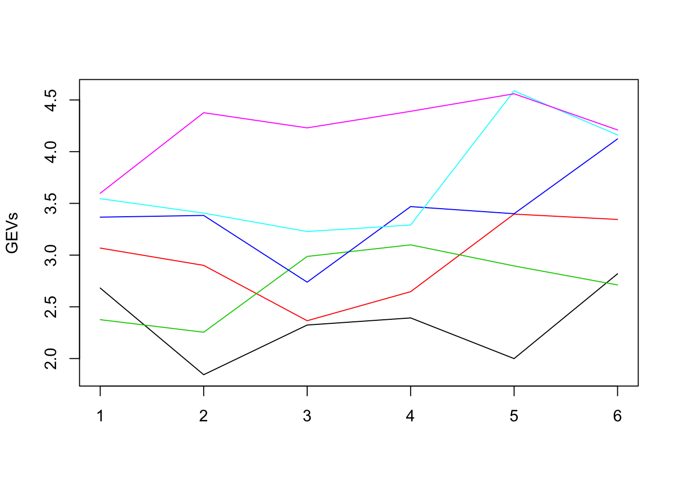
Define the host-specific effects distribution
The final phenotype of every infected host is the sum of the GE-value for its currently infecting strain and a random host-specific effect. The toyepidemic package assumes that the host-specific effect is a normally distributed random variable drawn exactly once for each possible infecting strain in a newly infected host. This normal distribution has mean 0 and standard deviation defined by the following parameter \(\sigma_e\):
# is the special environmental effect unique for each pathogen genoetype in an individual
eUniqForEachG <- TRUE

sigmae <- .6
# it is possible to specify different standard deviations for the different host-types, i.e. different host-types exhibit stronger or weaker effect on the trait. For this example we keep them fixed for all host-types.
sde <- rep(sigmae, n)
Defining the population parameters
At the between-host level we start by defining the size, the birth- and the natural death rate in the population at equilibrium. These are constants:
#initial population size (equilibrium in the absence of disease)
N <- 1e5

# setting the between-host and within-host dynamics of the simulation:
# natural death rate
mu <- 1/850

# constant birth rate that maintains this equilibrium
nu <- ifelse(is.finite(N), mu*N, 0)
Next, we define the rate parameters for infected hosts: ### Infected death-rate
# death-rate as a function of viral load and natural death rate mu
rateDie <- function(z, mu) {
  V <- 10^z
  Dmin <- 2
  Dmax <- 25*12
  D50 <- 10^3
  Dk <- 1.4
  (V^Dk+D50^Dk)/(Dmin*(V^Dk+D50^Dk)+((Dmax-Dmin)*D50^Dk)) + mu
}

curve(rateDie(x, mu), 0, 7, col="red")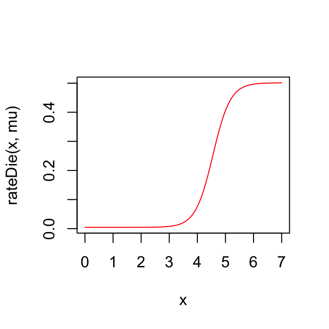
Transmission-rate as a function of viral load and rate of risky contacts with susceptible hosts
rateContact <- 1/6

# note that at runtime, rateInfect is scaled by the proportion of susceptible hosts
rateInfect <- function(z, rateContact) {
  V <- 10^z
  Emin <- .3
  Emax <- .6
  E50 <- 10^3
  Ek <- 1.4
  E <- Emin+(Emax-Emin)*V^Ek/(V^Ek+E50^Ek)
  E*rateContact
}

curve(rateInfect(x, mu), 0, 7, col="red")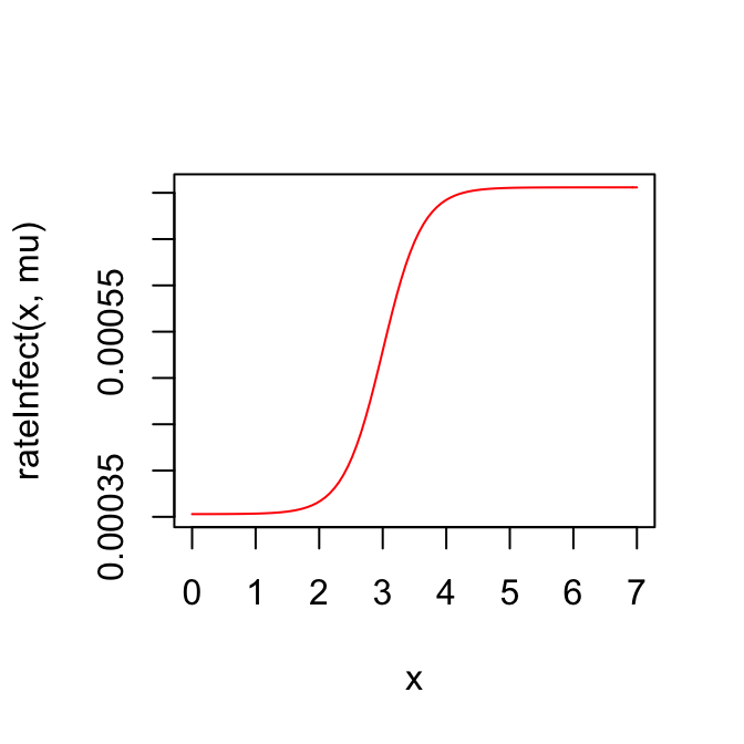
Within-host strain mutation rate
We define a function rateMutate which calculates the within-host per-locus mutation rate for a number K of infected hosts. The function recieves the GEVs matrix as an argument and 3 vectors of length K as follows:
- es: numeric : values of currently active host-specific effects;
- envs: integer : host types for the K infected hosts;
- genes: integer : currently infecting strains for the K hosts.
In addition, we specify the mode of within-host evolution (in this case - selection)
# per locus mutation rates
rateMutate <- function(GEValues, es, envs, genes) {
  z <- GEValues[cbind(envs, genes)] + es
  V <- 10^z
  Mmin <- 0.00
  Mmax <- 0.2
  M50 <- 10^3
  Mk <- 1.4
  Mmin+(Mmax-Mmin)*V^Mk/(V^Mk+M50^Mk)
}

# are only beneficial (i.e. increasing the trait-value) mutations allowed
selectWithinHost <- TRUEDefine the time step and the duration of the simulation
# all events are sampled with this time-step. This means that only one event can happen for an infected host within every next interval of 0.05 (arbitrary time units).
timeStep <- 0.05

# maximum time before starting graceful fadeout of the epidemic (stop the
# transmission events and wait until no more infected hosts live in the population)
maxTime <- 200

# continue the epidemic outbreak until reaching maxNTips diagnosed hosts
maxNTips <- 1000

# time to continue the simulation of transmission after reaching maxNTips
# (this was introduced in order to study post-outbreak dynamics, i.e. epidemic
# waves after exhaustion of the susceptible pool)
expandTimeAfterMaxNTips <- 0
Running the simulation
To run the simulation we use the function simulateEpidemic with the parameters specified as above:
epidemic <- simulateEpidemic(
  Ninit=N, nu=nu, mu=mu, pe=pe, sde=sde, pg.init=pg.init, GEValues=GEVs,
  rateContact=1/6, rateInfect=rateInfect, rateDie=rateDie,
  rateSample=rateSample,
  rateMutate=rateMutate,
  numsAllelesAtSites=numsAllelesAtSites, eUniqForEachG=eUniqForEachG,
  selectWithinHost=TRUE,
  timeStep=timeStep, maxTime=maxTime, maxNTips=maxNTips,
  expandTimeAfterMaxNTips=expandTimeAfterMaxNTips,
  process="select/select")
Analysing the epidemic
Here we glimpse over some of the functions used in analyzing the simulated epidemic. A more elaborate analysis is provided in the vignette for the package patherit.
Extracting the transmission tree connecting sampled host
tree <- extractTree(epidemic)## Generating tree: nTips= 1000 , number of uncollapsed edges= 3393plot(ape::ladderize(tree), show.tip.label = FALSE)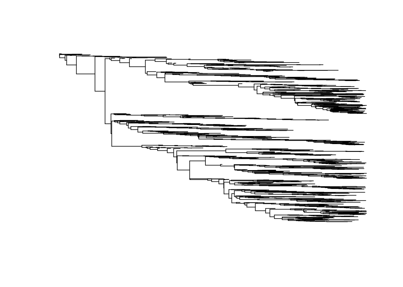
Extract the population of sampled patients
# extract the population of all sampled individuals
pop <- extractPop(epidemic, ids = tree$tip.label)

# calculate their phenotypic values at the moment of diagnosis
pop[, z:=calcValue(env, gene, e, GEValues = epidemic$GEValues)]

hist(pop[, z])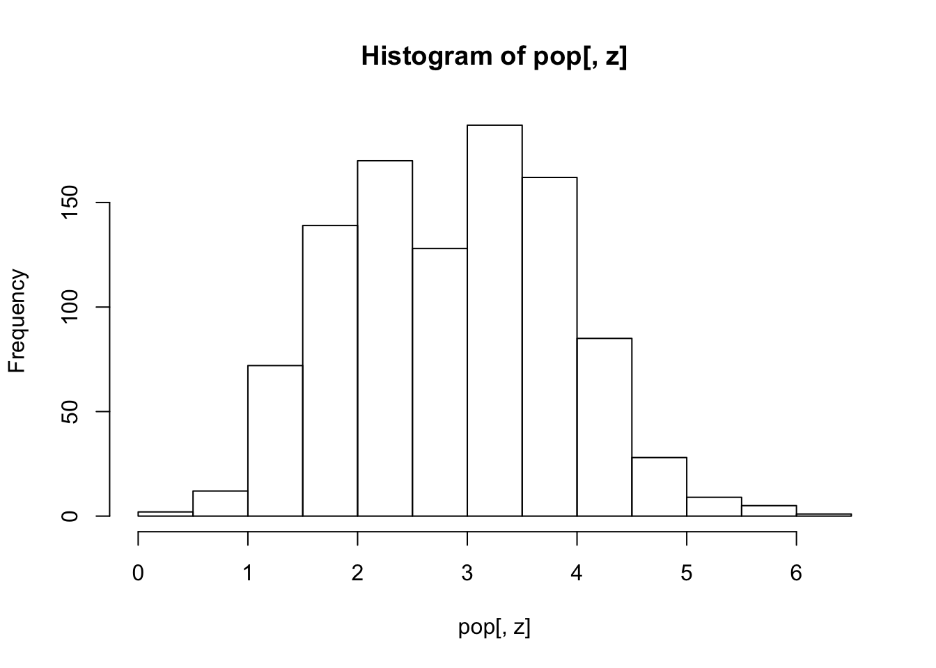
Extract donor-recipient couples
drc1 <- extractDRCouples(epidemic)Packages used
Apart from base R functionality, the toyepidemic package uses a number of 3rd party R-packages:
- For fast execution: Rcpp v0.12.14 (Eddelbuettel et al. 2017);
- For tree processing: ape v5.0 (Paradis et al. 2016);
- For reporting: data.table v1.10.4.3 (Dowle and Srinivasan 2016);
- For testing: testthat v1.0.2 (Wickham 2016).
Further reading
For a further introduction to the toy epidemiological model, we refer the reader to (Mitov and Stadler 2016).
References
Dowle, Matt, and Arun Srinivasan. 2016. Data.table: Extension of ‘Data.frame‘. https://CRAN.R-project.org/package=data.table.
Eddelbuettel, Dirk, Romain Francois, JJ Allaire, Kevin Ushey, Qiang Kou, Nathan Russell, Douglas Bates, and John Chambers. 2017. Rcpp: Seamless R and C++ Integration. https://CRAN.R-project.org/package=Rcpp.
Mitov, Venelin, and Tanja Stadler. 2016. “The heritability of pathogen traits - definitions and estimators.” Unpublished Data https://www.biorxiv.org/content/early/2016/06/12/058503.
Paradis, Emmanuel, Simon Blomberg, Ben Bolker, Julien Claude, Hoa Sien Cuong, Richard Desper, Gilles Didier, et al. 2016. Ape: Analyses of Phylogenetics and Evolution. https://CRAN.R-project.org/package=ape.
Wickham, Hadley. 2016. Testthat: Unit Testing for R. https://CRAN.R-project.org/package=testthat.